Monthly Archives: October 2012

Bike Accumulation at Hubway Stations

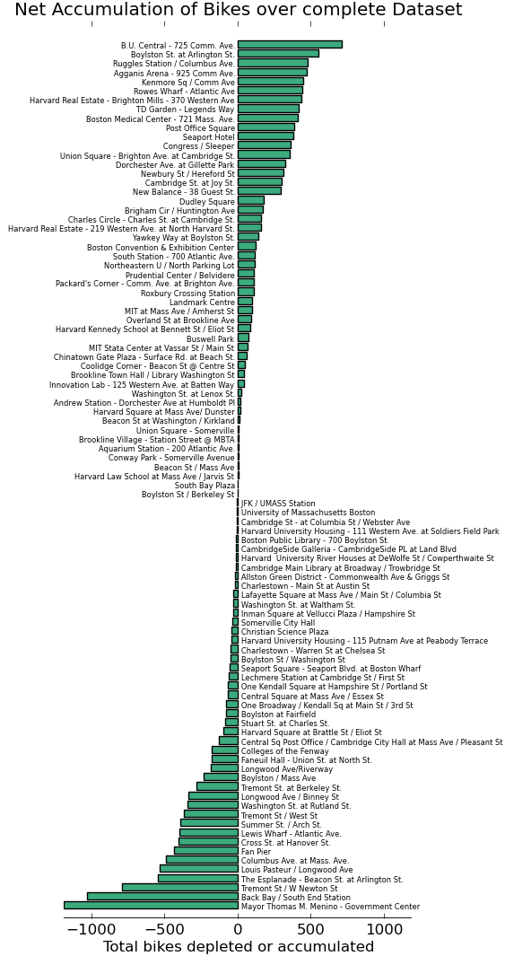
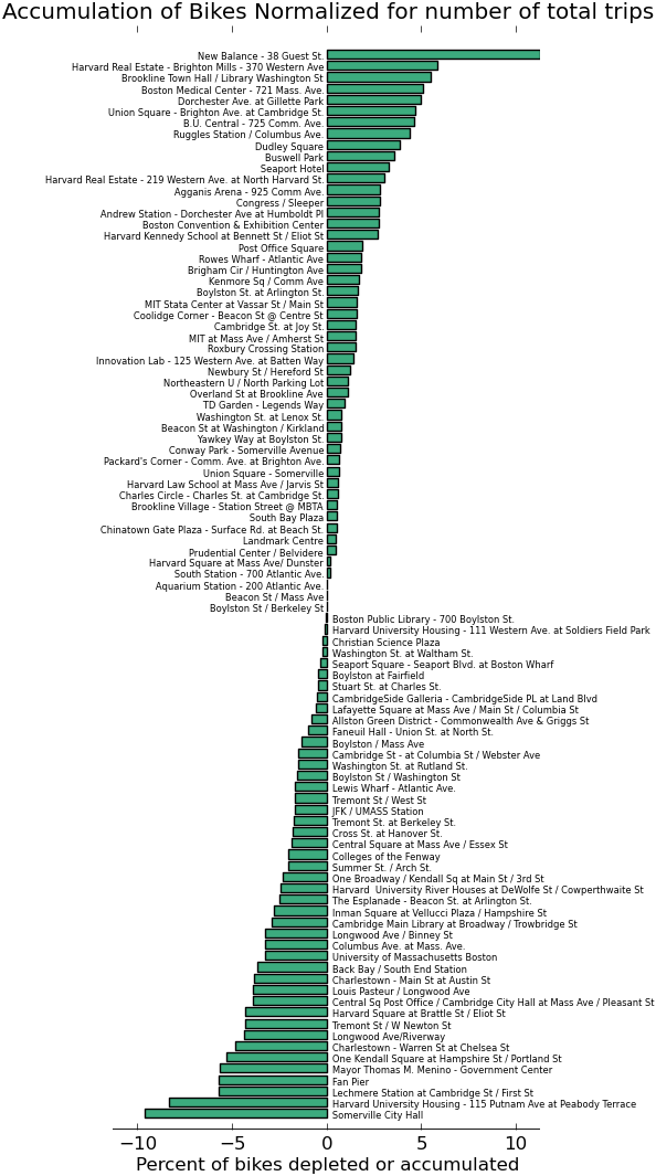
Looking at the whole dataset gives a sense of how much effort must be spent keeping bikes/empty space at different stations as needed. To some extent users are responsible for this because they have to leave the bike somewhere, which might mean going to further to an empty station.

The following shows the normalized accumulation of bikes as a percentage of the total number of trips from each station:

The following shows the net bike accumulation or depletion:

Hubway Trip Durations versus cost

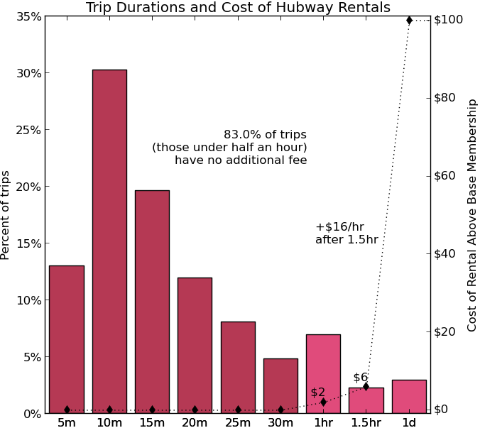
The Hubway bike rental specifically targets short trips, anything under 30 minutes is part of the membership fee (either a year, 3-day or 24 membership). This seems to suit most users, with 43% finishing within 15 minutes and 62% finishing in 20 minutes.

After the first 30 minutes additional fees are incurred (with a 20% discount for registered riders). The data below shows the % of trips with different durations and the fees an unregistered rider would incurr. Note that local bike rentals are around $40/day and Hubway even recommends places to go for longer rentals.

I also saw in a previous post that some trips are being made pretty much from all stations to all other stations, which I suspect means there are trips that can’t be easily made on a Hubway bike in traffic in 30 minutes.

Note, I would like to represent this data with a cumulative bar chart and something with the cost more proportional to the number of trips that paid it.

Hubway trips for August 2012

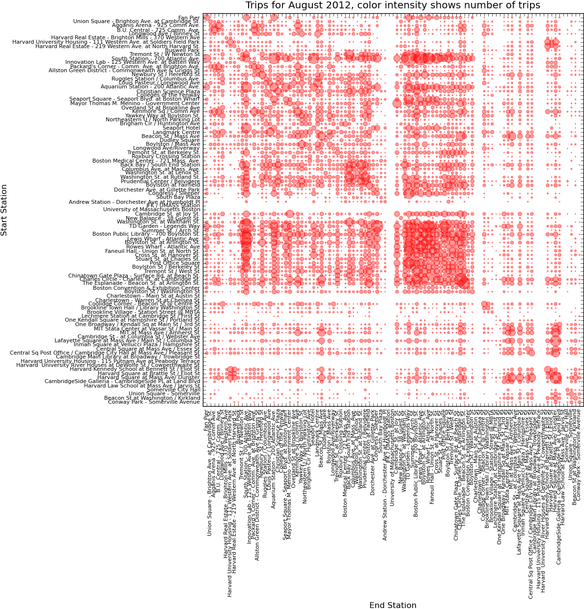
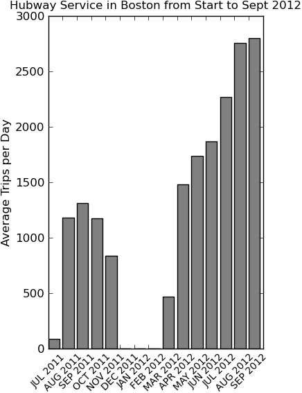
I took a closer look at the Hubway trips data for August 2012 data (busiest month on record with average of nearly 3,000 trips per day) and was surprised that almost all stations were connected by some trips. Also with clear clustering for TD Garden (North Station) and South Station, Harvard and the diagonal representing round-trip rentals. Other symmetry on the diagonal likely representing commuters going from one destination to another and back again later. The cluster on the diagonal over the whole data set highlights the 6.93% of trips which return to the same location.

This figure was generated with matplotlib and data processed in python. Unused stations were likely not opened yet in August.

Mapnik experiments

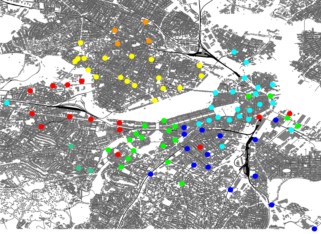
After a day of working with mapnik, I have my first supremely ugly plot, which shows Hubway station locations around Boston, the colors are by station name prefix, which is roughly by area, but not that logical outside Cambridge and Somerville…

Ha! Decided to try to add some color to these water bodies myself in the sytlesheet. Ended up coloring all of the following:

<Filter>[natural] = ‘water’ or [natural] = ‘lake’ or [natural] = ‘bay’ or [natural] = ‘wetland’ or [natural] = ‘marsh’ or [gnis:feature_type] = ‘Bay’ or [landuse] = ‘reservoir’ or [landuse] = ‘basin’ or [waterway] ‘canal’ or [waterway] = ‘boatyard’ or [wetland] = ‘wet_meadow’ or [wetland] = ‘tidalflat’ or [wetland] = ‘saltmarsh’ or [wetland] = ‘swamp’
</Filter>

Which still didn’t manage to get any of the Boston Harbor or the Mystic River, however, I am tabling it for a while.

Plot thickens and the cast weakens

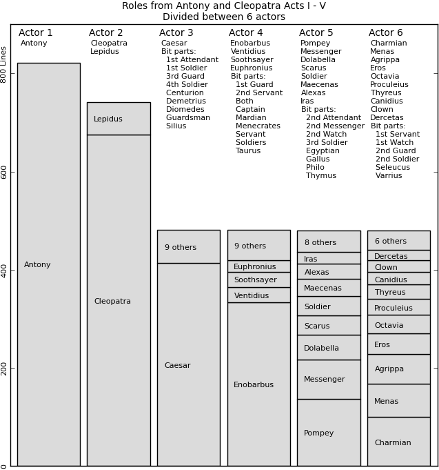
What ho, our Julius Caesar performance is now down to 3 or 4 people! Turns out still enough for a very fun evening:

The results are much less pleasing from my greedy algorithm. In the end we mostly used the allocation only for the large parts and just moved the smaller parts about as needed. It was pretty fun to completely ignore which commoner says stuff and just pass the dialog around naturally.

With 3 people:

With 4 people:

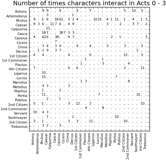
Here are the conflicts:

Gender demographic of Hubway users

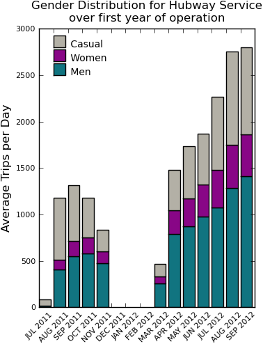
Looking at the gender distribution of users, the data is not very interesting. Aside from an initial ramp up as users registered in the first few months, things seem pretty stable at between 10-18% Women and ~50% Men with the rest unregistered (no gender information available).

I used cPickle to serialize my python representation of the data to store and retrieve the processed data. Useful to speed things up.


For the record below is the ugly default legend which looked terrible on the plot.

Julius Caesar – performing the play with a small cast

I have scheduled a dramatic reading of Shakespeare’s Julius Caesar with a small group of friends. The play has 46 speaking roles, but I expect only about 5 people at the reading and decided to try to divide up the roles equitably between my small cast. Goals:

  1. Evenly distributed number of lines between the actors.
  2. Try not to have the readers performing dialog with themselves.

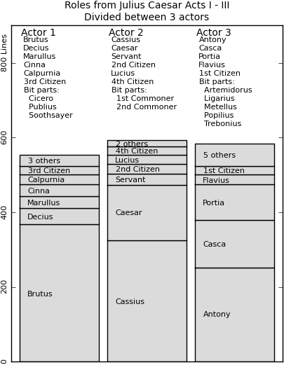
I extracted character, linecount and who-speaks-to-whom information about the play from the gutenburg project text version, which was very well formatted and made it quite easy. Here is the line count information for each of the 46 named speaking characters in the play. Note the names of the characters vary between versions: i.e. FIRST COMMONER = CARPENTER and SECOND COMMONER = COBBLER in different editions.
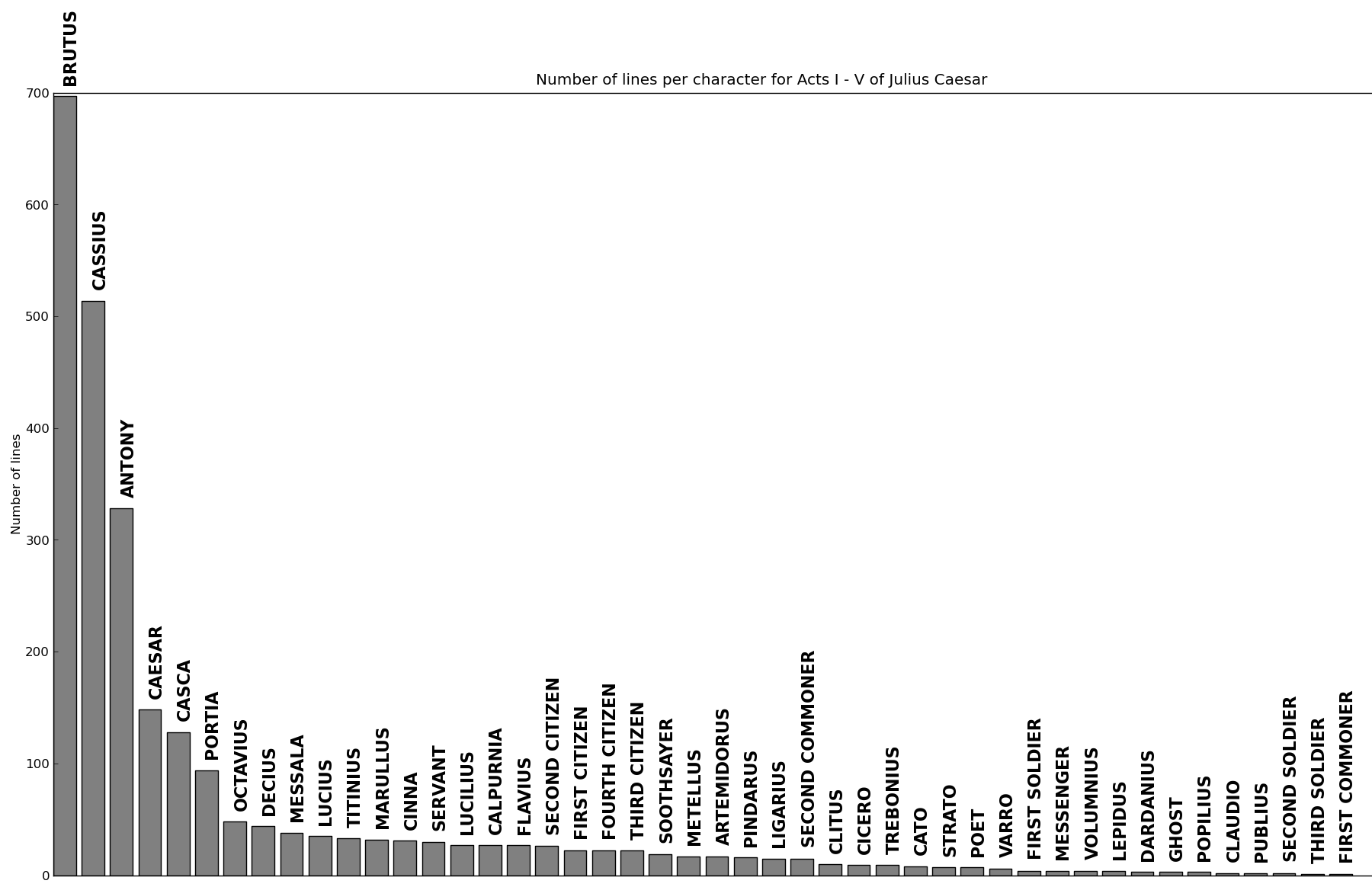
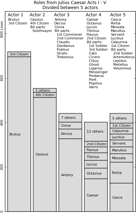
An equitable distribution for 5 characters would be ~500 lines per piece, since Brutus alone as 700 lines, he will always be the star in a 5 person performance.

Turns out the optimal solution is non trivial, being 5^46 total number of combinations, can’t test them all. However, it looks like I can defer the correct solution for now, since a greedy algorithm which takes each character in the play in the order of the most lines and assigns them to an actor with a cost function that attempts to distribute the lines evenly with a heavy penalty for talking to yourself seems to work well. With only 5 actors the whole play can be performed with someone talking to themselves only 3 times (not bad since I actually had to do that on stage in a play in 5th grade, much to the amusement of the crowd). The line distribution is fairly equitable for the non-Brutus and non-CASSIUS characters.
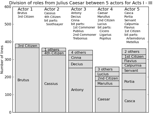
Fortunately, we are unlikely to read the whole play, so I will divide up the play for only the first three acts and see what happens, for these three acts there is one case of an actor delivering a line back-to-back with another character they are playing and the total cast is reduced to 27 characters.
The good news is if someone calls in sick or we have surprise guests, I can easily re-allocate the roles. Not optimal, but passable for this event.
Reading HTML with Python

Today I read some HTML data from a table using Python. The tools I ended up using to get the data were:

import urllib
f = urllib.urlopen(<URL_string>)
# Read from the object, storing the page's contents in 's'.
s = f.read()
f.close()

Then to parse tables in the HTML I used lxml which can read HTML and provide an ElementTree like API.

from lxml import etree
html = etree.HTML(s)

I was then able to do everything I needed using list() on the element to get the children and using the attributes .text and .tag to get the text out of tables and links as desired.