As winner of Best Analysis in the 37 Billion Mile Challenge, our team came home with the VMTWIZ vanity plate:

For the uninitiated (myself included before working with Paul on this project), VMT stands for Vehicle Miles Traveled. I finally put it up on my wall of inspiration today!

I ran into an interesting problem updating a legend rendered with d3 today. I am displaying different data sets on a map and adjusting the colors and cutoff values based on what variable is selected. The image below shows two example states of the legend, the third is the unexpected result when I transition from the first to the second and the “200-300″ case fails to update.

My data for the legend was structured as a list of lists:

var legendStrings = [
    [" < 25", "25 - 50", "50 - 100", "100 - 150", "150 - 200", 
     "200 - 300", "300 - 400", "400 - 500", "   > 500"],
    [" < 10", "10 - 50", "50 - 75", "75 - 100", "100 - 200", 
     "200 - 300", "300 - 500", "500 - 1000", "   > 1000"] 
];

In the legend update function I selected the appropriate legend string list from “legendStrings” based on the index of the data being displayed and attempted to create an appropriate compare function as discussed previously. However, this failed as shown in the picture above:

function updateLegend(ind /* index of variable being plotted */){

    var lstr = legendStrings[ind];
    var rects = legend.selectAll("rect")
         .data(lstr, 
              /* this compare function doesn't work, 
                 using "ind" here will have no effect. */
              function(d, i){ return d + ind*10 + i;});

    /* do the rest of the work to render rects, text, etc */
    /* then don't forget to remove exiting elements */
    rects.exit().remove();
}

My not so clever compare function included the index of the data, “ind”, so I thought it would enter new elements whenever the index was changed. However, this doesn’t work, because the compare function used is not bound to the data. So when update is run, the new compare function is used to compare the old data with the new data and the old compare function doesn’t exist anymore… The solution is to only use the attributes of your data (stored in d, and i) in the compare function, so in this case refactor the data representation so that it includes information about which variable is being stored. Or, you can always delete the elements and re-render them:

legend.selectAll("rect").remove(); 
/* then render new elements as above */

Which seems about the same to me in this case and was certainly a lot simpler. I guess I am still waiting to see the use case where I get excited about the d3 enter and exit functionality…

I am looking into using d3 in conjunction with Leaflet and worked through Mike Bostock’s tutorial on d3 and leaflet. Using the MAPC provided shapefile for municipalities, so far it seems really slow on zoom, I think because of the super high resolution shapes being recalculated. Check out the shape of Boston!

Can I just say that Boston is genuinely a weird shaped town? I particularly love these oddities:

1. The tiny sliver in of Boston that extends into Everett!
2. A small section of the airport is in Winthrop
3. The tail end of Winthrop peninsula is in Boston
4. Brookline. Need I say more…

I was having some trouble visualizing the geoJSON files I generated in the previous post in d3. Does this look like Somerville in blue to you? No?! Well obviously the pink is Cambridge though…

Turns out the problem was the wrong projection. The MAPC data (or most of it) is using the NAD83(HARN)/Masssachusetts Mainland EPSG:2805 (QGIS reports this), also known as,  “NAD_1983_StatePlane_Massachusetts_Mainland_FIPS_2001″ from the .prj in the shape file.

Apparently, pyshp doesn’t handle reading the .prj files very well, it kinda ignores them on purpose (https://code.google.com/p/pyshp/issues/detail?id=3). So using pyshp to convert the shapfiles to GeoJSON probably wasn’t a good choice (no projection info will be transferred to the GeoJSON).

GeoJSON allows for specifying a CRS, but assumes use of the default of WGS84 if none is specified according to the spec. I tried to explicitly set the CRS in the geoJSON, but that doesn’t seem to be working, it looks like the d3 code is ignoring the “crs” property and assuming WGS84 as well.

I then tried saving the layer as GeoJSON with QGIS (version 1.7.5), despite the very nice save dialog and carefully selecting the desired projection, it doesn’t work at all:

1. The GeoJSON was not reprojected to the desired coordinate system (pretty similar to this reported QGIS issue), and
2. QGIS does not populate the crs property in the output GeoJSON

However, saving the layer as an ESRI shapefile you can change the projection using QGIS.

I was able to use ogr2ogr to convert the GeoJSON generated by pyshp with no CRS specified to WGS84 (“EPSG:4326″), after which it renders correctly in d3. (Note when I tried different target projections there was still no crs property in the GeoJSON! It looks like support for different crs in GeoJSON is pretty spotty). Here is the ogr2ogr command I used for the simple projection change:

ogr2ogr -f "GeoJSON" -t_srs "EPGS:4326" -s_srs "EPGS:2805" new.geojson old.geojson

And now you might recognize these Boston suburbs:

At this point really what is the point of using any tool other than ogr2ogr? For example, the following command converts the Massachusetts municipalities shape file to GeoJSON, reprojects it correctly, and filters out all the cities except cambridge and somerville.

ogr2ogr -f "GeoJSON" -t_srs "EPSG:4326" \
        -where "municipal IN ('CAMBRIDGE','SOMERVILLE')" \
        camberville.geojson \
        ma_municipalities.shp

All in one command and it does it correctly (although ogr2ogr doesn’t seem to put crs info in the geojson either, so I’d stick with WGS84 as much as possible).

Do you want to animate a line so that it looks like it is being drawn on the screen?

At a first pass you might think this would be difficult, for example requiring you to draw in the path piecemeal like this: https://groups.google.com/forum/#!topic/d3-js/pWOfEThcnIg Ugh!

However it turns out it is trivial if you use the svg stroke properties: stroke-dasharray and stroke-dashoffset as demonstrated in this bl.ock and discussed below. The trick is to understand how the dasharray and dashoffset work.  The dasharray is a list of lengths that specify alternating dashes and gaps, starting with a filled section (you can create all sorts of dash-dot patterns). The offset shifts the pattern start point to the left. Here is a quick example I drew in Inkscape, as an experiment in exploring SVG through an SVG drawing program. I was disappointed that the concepts here are abstracted away by the GUI (might as well be drawing it in Word), but by inspecting the output svg file I was able to determine the values being used in the image below for the stroke-dasharray are “48,48” and the stroke-dashoffsets are “24” and “48”. For this example only the ratios are relevant.

Now, in order to use these properties to animate a line draw:

1. Calculate the length of the rendered line (or bigger works too for this example), call it lineLen for this example.
2. Initialize the line with a stroke-dasharray of “lineLen, lineLen”, so the filled dash and the gap are each greater than or equal to the length of the line.
3. Initialize the stroke-dashoffset to “lineLen” so that the pattern will start with a gap (your line will start invisible).
4. Transition the stroke-dashoffset to zero, this will cause the pattern to shift to the right, revealing your line from the left to the right (moving from the bottom up in the example above).

Here is the key bit of code, assuming you know some d3 and have some “data” and a “line” defined for it.

   var path = svg.selectAll("path")
        .data(data)
        .enter()
        .append("path")
        .attr("d", line)
        .attr("fill", "none");

   var lineLen = path.node().getTotalLength(); // 1. get length

   path.attr("stroke-dasharray", // 2. pattern big enough to hide line
                   lineLen + ", "+lineLen) 
        .attr("stroke-dashoffset",lineLen); // 3. start with gap
   path.transition()
        .duration(2000)
        .attr("stroke-dashoffset", 0); // 4. shift pattern to reveal

Here is a bl.ock playing around with an absurd progress bar concept (not really), but having fun with other dasharray patterns: http://bl.ocks.org/zsobhani/9236015

I used this trick to draw a line on the screen as an enter animation on recent project and loved the simplicity of the solution.

I was expecting the task of adding labels to the treemap to be pretty arduous, but it ended up being simpler than I expected.

Step 1: Determine the size of the label and if it will fit in the box:

This zoomable treemap demo provided an example of how to put labels only on the boxes that are big enough for them. Before looking at this code I wasn’t aware of the svg function .getComputedTextLength(), which tells you how big the text renders. What a life saver, no need to worry about font style or size! In my case, I also needed to know the height of the box, which means I ended up using .getBBox() which gives both the height and the width for a text element (where the width is the same as what is returned by .getComputedTextLength()). The downside of .getBBox() is you have to render the element, you can’t check before creating the label. I am handling this similar to the demo code above, by simply setting the opacity of the text based on whether it fits in the box.

• First, center the text over the box by setting x, y as the center of the box and using text-anchor:middle

.attr("dy", ".35em")
.attr("text-anchor", "middle")

• Then set the opacity to 1 if the text fits in the box and 0 otherwise:

.style("opacity", 
    function(d){
       bounds = this.getBBox();
       return((bounds.height < d.h -textMargin) && 
              (bounds.width < d.w-textMargin)    ) ? 1:0;
     })

Now there are labels on everything, but the labels on the small cells are invisible!

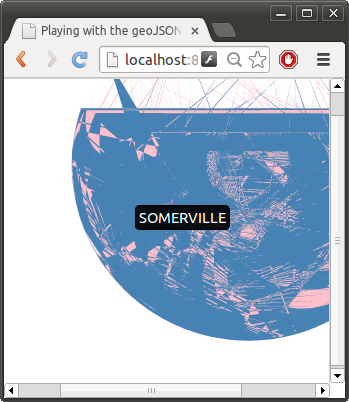
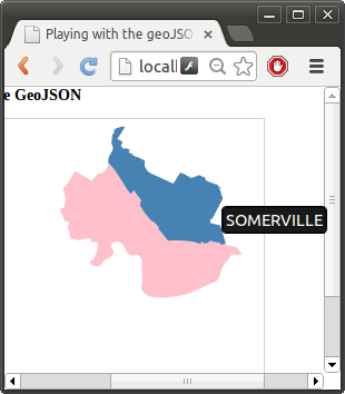
Step 2: Fix mouseover so that tooltips and box highlighting continues to work with new text labels

The text over the tree boxes by default grabs the mouse cursor and changes it to a edit icon (this can be seen in the d3 example above). Even more annoying it grabs the mouse events so that the tooltips are virtually impossible to see anymore. Especially since the invisible (opacity 0) labels can be quite long and larger than the cell on small data points. I found an excellent discussion of SVG mouseover by Peter Collingridge. These mouseover issues were cleanly solved by setting the css to “pointer-events: none;”

Step 3: Adjust color of text based on background color

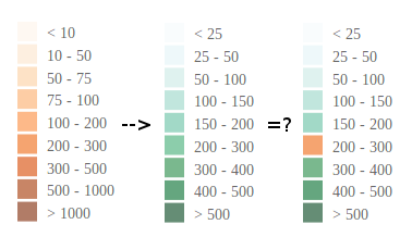
I still haven’t found a good solution for this feature. Ideally as a designer I would want to specify a HSL color threshold to switch between white and black text, however, I don’t think it is possible to get the color value corresponding to this HSL threshold out of the d3.interpoloateHsl(), so I unfortunately have to set the color threshold (using the input units) manually… For example, something like this:

.attr("class", function(d){
    return (d.colorRaw < 0.07) ? "tree-label-dark" : "tree-label-light";
})

where d.colorRaw is the color metric scaled to HSL using the d3 interpolation.

I would much prefer to specify three HSL values, 2 for the range and a third threshold value to switch the label class from “dark” to “light”, but I’m still not sure how to do this. Is there a way to reverse out the number that generates something on the HSL scale? Or compare HSL values?

Note, I love this HSL color picker. Since it provides steps I think it would be very easy to pick a threshold value in the right space…

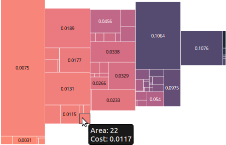
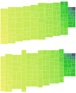
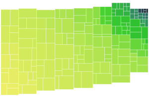
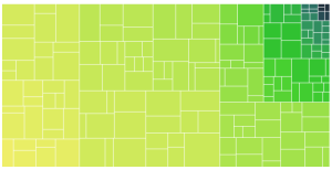
Final example with working labels:

The labels displayed are simply the raw color data. Notice how the mouse over tooltip is working on a cell with no label.

Continuing the work on the Color Prioritized Tree Map, I implemented variable column widths as a step towards making the tree map look more organic. The top picture here is uniform widths for reference and the one below introduced some variable widths, specifically I used a widths multiplier array of [2,3,4,2,5], which is then wrapped to apply a multiplier to the width of each column. This means the second column is 50% wider than the first etc.

The column widths are assigned before the data is binned, the bin sizes are now equal height instead of equal area. Below is another example. Based on initial testing, the variable widths improve the image best when tweaked and evaluated by eye (since the data set and number of columns also affect the resulting shape). Overall, variable column widths were not as big a gain as I was hoping. Also since the columns are centered on a diagonal, the stepping appearance is retained. I guess introducing variable height would help! But I think the better approach is to look into ragged edges first.

I also tested out a few other data sets, these ones are really lumpy:

I am still not sure what sort of data will be representative for the target application, but these data sets did stress the viz a bit and demonstrated that the following suspected issues are real:

• Very small areas erased by a white border: The border is implemented by subtracting a “margin” value from the desired length and width of each element and may result in invisible cells for very small areas. In practice these are so small as to be virtually invisible before, but I modified the code to not apply the white space if it will erase the data point for now.
• Bad data in the form of missing fields crashes the viz: This is corrected now handled by silently rejecting those data points.
• Giant elements overflow the column and go off the top of the user provided SVG: Elements with area greater than what should be in a column get put in a column anyway, in which case, the tree map can go off the top of the SVG. It probably makes sense to have some guidelines regarding number of columns based on the size of the largest data and the distribution. A related improvement would be to verify that we aren’t drawing outside the designated box and scaling everything down appropriately if we are to ensure we stay on the user provided SVG.

Continuing the color prioritized treemap project, I built an appropriate tree data structure, where each Node represents either

• a leaf
• a group of Nodes (horizontal groups constrained to have the same width and vertical groups to share height)

Important methods include:

• getArea() which returns the total area for all children
• createSubGroups() which performs the grouping on this node’s node-group (creating the tree), and
• flatten() which takes the start coordinates of lower left corner and height or width constraint and recursively flattens the tree, returning a list of boxes with fully defined coordinates appropriate for d3 rendering of the tree map.

To retain the overall organic shape, the highest level is represented as separate columns, each as a vertical node group (if these columns together were considered a horizontal group, the overall shape would be square). I restructured the previous example to use my new data structure. The following screen shot demonstrates that horizontal and vertical grouping is working, as well as the rendering code. As a basic test I simply grouped the first 6 Nodes in the column into a horizontal group:

The overall shape here is unchanged from before, you can see that the order of Nodes (defined by the gradient) is retained.

Next up: working on the algorithm for which Nodes to group and how, and thus create a pleasing shape.

The following screen shot shows some great improvements and some simplification of the approach too. Now for each column, the elements are grouped into a tree structure, where the smallest area node in a group is paired with the smaller of its neighbors (building a tree of fairly balanced area at each level). Now when flattening the tree, the node groups are assigned either vertical or horizontal orientation based on which will give the better aspect ratio for the sub-groups based on the dimensions of the block being filled. This is the data now with 8 columns:

It seems to be shaping up nicely, but would be good to fray the edges and vary the column widths to mask the columns better (as Mark Schindler noted, they imply a structure to the data that is not there).

For curiosity’s sake, here is the same data with only one column. What looks kinda like 3 columns here is an artifact of the grouping algorithm (at each level the data is divided in groups), data set and svg aspect ratio:

Now, it’s time to try out a few different data sets and see what other issues shake out.

The Jaybridge Challenge 2013 is now over and from a technical perspective it went flawlessly. I am pretty thrilled with the performance of the site. The challenge itself was interesting, a well designed problem that allowed a wide range of solutions. The only downside was the small number of contestants. I would estimate 1/50 people who learned about the competition looked at the site and about 1/50 of those signed-up. Of those 1/2 submitted a solution. So for next time, plan on spending more effort on publicity and perhaps time the competition with school holidays of some sort.

Adding Fields to the live database:

During the competition I discovered a bug in my calculation of the leaderboard rank for tied scores (which occurred since the trivial solution generates a repeatable score and pretty much everyone will log that for their first score). Instead of using the submission time to differentiate the leader in case of a tie, I was using the user’s signup time. During beta testing, users signed up and then got a trivial solution in a short time, so the sorting appeared to work fine. When I noticed the bug during the competition, I realized is should have been tracking the submission time along with the submission id and score in the best score database. Making this change on the live site required adding some fields to the database, which was a bit scary, since I hadn’t tried something like this before. (In retrospect, I would say that it’s pretty similar to lots of backwards compatibility things I’ve done in the embedded world. I like when that stuff translates.)

Code Steps:

1. Add new field to the entity constructor
2. Write a function to “massage the db”, adding in values for the new field to entries that don’t have it and create a handler from some url to trigger this massage.
3. Update the leaderboard code to use the new database field.

Test Deployment Steps:

I tested the changes as I went on my development server and all seemed to be going well. I then deployed the change on our beta-test site and discovered several problems (the first 2 related to the initial default values not apparent on development server tests):

1. Corner case of best_score == 0 wasn’t handled correctly (because in my test submissions I hadn’t realized this was a valid score.)
2. Invalid submission id’s not checked for.
3. The leadboard queries stopped working for a time, while the new database indexes were building, making the site nonfunctional for a few minutes, which I deemed unacceptable.

Live Competition Site Deployment:

Based on the test site deployment, I fixed the 2 bugs and then broke the deployment down into a few steps as follows.

1. Deploy to the live site the changes to the db constructor and the massage functionality only.
2. Hit the “massage db” url, so that all new data in the db is populated and wait a bit for indexes to be created.
3. Deploy the change to the leaderboard to use the new database information.

And wallah! Flawless deployment, I was pretty grateful to have the extra layer of testing provided by our beta-test site. It was definitely kinda scary to risk a change like this while the competition was live, but it went very well and I learned something about making db changes like this, enough to get this job done.

A note on cost:

Regarding the operating cost/optimization/developer time trade-offs it was interesting to see the challenge didn’t get enough interest to run up any significant costs. We did accrue ~10 cents of database queries beyond the free quota. I definitely hadn’t anticipated the number of submissions that some contestants would make. Some appeared not to be doing any basic validation on their submissions locally (I suppose some didn’t have Ubuntu VMs to test on and didn’t think to set them up), which meant for one Java user ~90 submissions which failed to execute in some way before getting a score. One team used some randomness in their algorithm and so would submit the same entry multiple times for different scores, with nearly 250 submissions in total. I wasn’t caching the table of each users submissions, even if I had I probably wouldn’t have thought initially to incrementally update the cached value and minimize the big queries, since it hadn’t occurred to me that any single user would make so many submissions, certainly none of our beta testers did. Here are screenshots of the submission history for the users mentioned above (scores anonymized):

In the end not spending time optimizing was of course the right thing, since none of that was needed. Also I would have guessed wrong about where the high use was going to be.